This yields the subgrid-scale stress, which is inserted in the momentum equation:

//pimpleFoam_with_sensor_sgs_model/Ueqn.H

MRF.correctBoundaryVelocity(U);

tmp<fvVectorMatrix> tUEqn

(

fvm::ddt(U) + fvm::div(phi, U)

+ MRF.DDt(U)

+ turbulence->divDevReff(U)

+ fvc::div(tau_sensor)

==

fvOptions(U)

);

fvVectorMatrix& UEqn = tUEqn.ref();

UEqn.relax();

fvOptions.constrain(UEqn);

if (pimple.momentumPredictor())

{

solve(UEqn == -fvc::grad(p));

fvOptions.correct(U);

}

Through the subgrid-scale viscosity, further closure terms can be determined by means of the gradient flux approach. For example, the implementation of the subgrid-scale thermal diffusivity within the energy equation could look as follows: 

alphat = nu_turbulent_sensor/Prt;

alpha_eff = thermo.alpha() + alphat;

In this example, Prt is the turbulent Prandtl number, which describes the ratio of the subgrid-scale viscosity to the subgrid-scale thermal diffusivity.

To check and facilitate the model’s implementation in your custom-built OpenFOAM® solver, we provide the code based on the pimpleFoam solver and an associated test case that represents the computationally inexpensive Taylor-Green vortex. The solver is based on OpenFOAM-v2006 and the source code has to be compiled with wmake before starting the simulation.

When conducting the simulation of Taylor-Green vortex, the flow field in the triply periodic box of side length 2 π  can be initialized by the setExprFields utility. Imposing the boundary conditions (type cyclic) and meshing (e.g. 32 x 32 x 32 uniform grid defined in system/blockMeshDict) are straight-forward in this case. 

The temporal evolution of domain-averaged kinetic energy and sensor statistics are monitored as follows. First, the corresponding fields are defined in createFields.H:

//Definition of Kinetic Energy

volScalarField KE

(

IOobject

(

"KE",

runTime.timeName(),

mesh,

IOobject::NO_READ,

IOobject::NO_WRITE

),

0.5*(mag(U)*mag(U))

);

//Domain-Averaged Kinetic Energy

scalar avgKE = KE.weightedAverage(mesh.V()).value();

//Domain Maximum of the Coherent Structure Function

scalar maxSensor = 0.0;

//Domain Maximum of the Sensor Function

scalar maxSensorFunction = 0.0;

//createFields for sensormodel

#include "createFields_LES.H"

Then, in the header of the main solver file pimpleFoam_with_sensor_sgs_model.C, the following output streams are defined:

//define output stream for kinetic energy

fileName outputFileKE("avgKE");

OFstream osKE(outputFileKE);

//define output stream for coherent structure function statistics

fileName outputFileSensor("structureFunction");

OFstream osSensor(outputFileSensor);

//define output stream for sensor function statistics

fileName outputFileSensorFunction("sensorFunction");

OFstream osSensorFunction(outputFileSensorFunction);

Finally, the quantities are calculated and written out within the time loop of the solver:

//On-the-fly kinetic energy calculation and output

KE = 0.5*(mag(U)*mag(U));

avgKE = KE.weightedAverage(mesh.V()).value();

Info << "Kinetic energy domain average = " << avgKE << nl << endl;

osKE << runTime.timeName() << "\t" << avgKE << endl;

//On-the-fly global maximum of the coherent structure function

maxSensor = 0.0;

maxSensorFunction = 0.0;

forAll(F, celli){

maxSensor = max(F[celli],maxSensor);

}

forAll(sensorFunction, celli)

{

maxSensorFunction =

max(sensorFunction[celli],maxSensorFunction);

}

reduce(maxSensor, maxOp<scalar>() );

Info << "Coherent structure function F domain maximum = " << maxSensor << nl << endl;

osSensor << runTime.timeName() << "\t" << maxSensor << endl;

reduce(maxSensorFunction, maxOp<scalar>() );

Info << "Sensor function domain maximum = "

<< maxSensorFunction << nl << endl;

osSensorFunction << runTime.timeName() << "\t"

<< maxSensorFunction << endl;

After the successful run of the Taylor-Green vortex simulation, your results for the global kinetic energy should be similar to the profiles in the figure below:

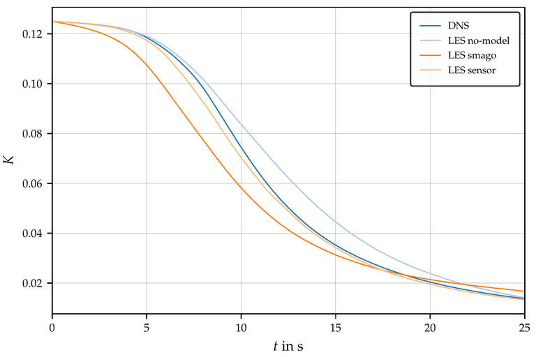
The convective and diffusive fluxes were evaluated by second-order central schemes. Temporal advancement was achieved by the second-order Crank-Nicolson scheme. In order to avoid masking of the results by numerical dissipation due to temporal discretization, it has been ensured that the Courant number is always below the value of 0.1. The sensor constant C_sensor = 1/0.16 used here is the same as in the original publication mentioned above but it may be worthwhile to recalibrate it for the specific test filter in OpenFOAM®.